Usage
The binary files above provide the required MATLAB binary libraries to reproduce the calculations presented in our publications as well as to conduct your own simulations.We provide two user interfaces to our code: A native interface (indicated by the ML prefix) and an interface that tries to replicate the function calls of FOCUS. If you use the FOCUS interface, ensure that you have FOCUS installed and running on your machine. In case of OSX, where no FOCUS binaries are provided, our functions can be used to replace some of FOCUS' functionality. The examples below only use FOCUS' MATLAB files and do not rely on the binaries.
The code shown in blue boxes shows our native interface, the code shown in green boxes uses FOCUS' interface.
Rectangular Piston
Get information about the interface:
MLRectangularPistonGrid
??? Error using ==> MLRectangularPistonGrid
Must have five or six input arguments: ([4x4 transform], [sx, sy, sz], l, s, k, ['cuda'|'cudadp'|'cpu'|'cpusp'|'cpudp'], [nabscissas])
Compute the near-field in front of a piston:
??? Error using ==> MLRectangularPistonGrid
Must have five or six input arguments: ([4x4 transform], [sx, sy, sz], l, s, k, ['cuda'|'cudadp'|'cpu'|'cpusp'|'cpudp'], [nabscissas])
%% setup the basic parameters
f0=1540000; % excitation frequency (Hz)
c=1500; % speed of sound (m/s)
lambda = c/f0; % wavelength (m)
k=2*pi/lambda; % wavenumber (1/m)
rho=1000; % acoustic density
%% setup piston parameters and the computational grid
s=5.0*lambda; % piston width
l=7.5*lambda; % piston height
siz = [ 61 1 101 ]; % grid sizes
sampling = [s/2/(siz(1)-1)/2*3 1 s*s/4/lambda/(siz(3)-1)];
transform = [ sampling(1) 0 0 0; 0 sampling(2) 0 0; 0 0 sampling(3) 0; 0 0 0 1 ];
%% do the calculation
pressure = MLRectangularPistonGrid( transform, siz, l, s, k, 'cuda', 40)*(1j*c*rho);
%% display and store the result
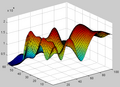
figure(1); surf(abs(squeeze(pressure))); axis tight
saveas(figure(1), 'figure1.png')
f0=1540000; % excitation frequency (Hz)
c=1500; % speed of sound (m/s)
lambda = c/f0; % wavelength (m)
k=2*pi/lambda; % wavenumber (1/m)
rho=1000; % acoustic density
%% setup piston parameters and the computational grid
s=5.0*lambda; % piston width
l=7.5*lambda; % piston height
siz = [ 61 1 101 ]; % grid sizes
sampling = [s/2/(siz(1)-1)/2*3 1 s*s/4/lambda/(siz(3)-1)];
transform = [ sampling(1) 0 0 0; 0 sampling(2) 0 0; 0 0 sampling(3) 0; 0 0 0 1 ];
%% do the calculation
pressure = MLRectangularPistonGrid( transform, siz, l, s, k, 'cuda', 40)*(1j*c*rho);
%% display and store the result
figure(1); surf(abs(squeeze(pressure))); axis tight
saveas(figure(1), 'figure1.png')
%% setup the basic parameters
f0=1540000;
define_media;
lambda = lossless.soundspeed/f0;
%% setup piston parameters and the computational grid
s=5.0*lambda;
l=7.5*lambda;
siz = [61 1 101];
sampling = [s/2/(siz(1)-1)/2*3 1 s*s/4/lambda/(siz(3)-1)];
ps=set_coordinate_grid(sampling,0,1.5*s/2,0,0,0,s^2/4/lambda);
transducer=get_rect(s/2, l/2, [0 0 0], [0 0 0]);
%% do the calculation
pressure=gpu_fnm_call(transducer,ps,lossless,40,f0,0);
%% display and store the result
figure(1); surf(abs(squeeze(pressure))); axis tight
saveas(figure(1), 'figure1.png')
This should result in a picture file called "figure1.png" that looks as follows:f0=1540000;
define_media;
lambda = lossless.soundspeed/f0;
%% setup piston parameters and the computational grid
s=5.0*lambda;
l=7.5*lambda;
siz = [61 1 101];
sampling = [s/2/(siz(1)-1)/2*3 1 s*s/4/lambda/(siz(3)-1)];
ps=set_coordinate_grid(sampling,0,1.5*s/2,0,0,0,s^2/4/lambda);
transducer=get_rect(s/2, l/2, [0 0 0], [0 0 0]);
%% do the calculation
pressure=gpu_fnm_call(transducer,ps,lossless,40,f0,0);
%% display and store the result
figure(1); surf(abs(squeeze(pressure))); axis tight
saveas(figure(1), 'figure1.png')
Circular Piston
If you want to compute the circular piston described in McGough's paper on the cpu, then use
MLCircularPistonGrid
??? Error using ==> MLCircularPistonGrid
Must have four or five input argument: (transform4x4, [sizex, sizey, sizez], radius, k, [, 'cuda' | 'gpu',[ abscissas]]
with the following parameters
??? Error using ==> MLCircularPistonGrid
Must have four or five input argument: (transform4x4, [sizex, sizey, sizez], radius, k, [, 'cuda' | 'gpu',[ abscissas]]
f0=1000000; % excitation frequency
c=1500; % speed of sound
lambda = c/f0; % wavelength
k=2*pi/lambda; % wavenumber
radius=5.0*lambda; % piston radius
siz = [ 61 1 101 ];
sampling = [1.5*radius/(siz(1)-1) 1 radius^2/lambda/(siz(3)-1)];
transform = [ sampling(1) 0 0 0; 0 sampling(2) 0 0; 0 0 sampling(3) 0; 0 0 0 1 ];
rho=1000;
pressure = MLCircularPistonGrid( transform, siz, radius, k, 'cpu', 40)*(1j*rho*c);
figure(2); surf(abs(squeeze(pressure))); axis tight; view(225,45);
saveas(figure(2), 'figure2.png')
f0=1540000;
define_media;
lambda = lossless.soundspeed/f0;
radius=5.0*lambda;
siz = [61 1 101];
sampling = [1.5*radius/(siz(1)-1) 1 radius^2/lambda/(siz(3)-1)];
ps=set_coordinate_grid(sampling,0,sampling(1)*(siz(1)-1),0,0,0,sampling(3)*(siz(3)-1));
transducer=get_circ(radius, [0 0 0], [0 0 0]);
pressure=cpu_fnm_call(transducer,ps,lossless,40,f0,0);
figure(2); surf(abs(squeeze(pressure))); axis tight; view(225,45);
saveas(figure(2), 'figure2.png')
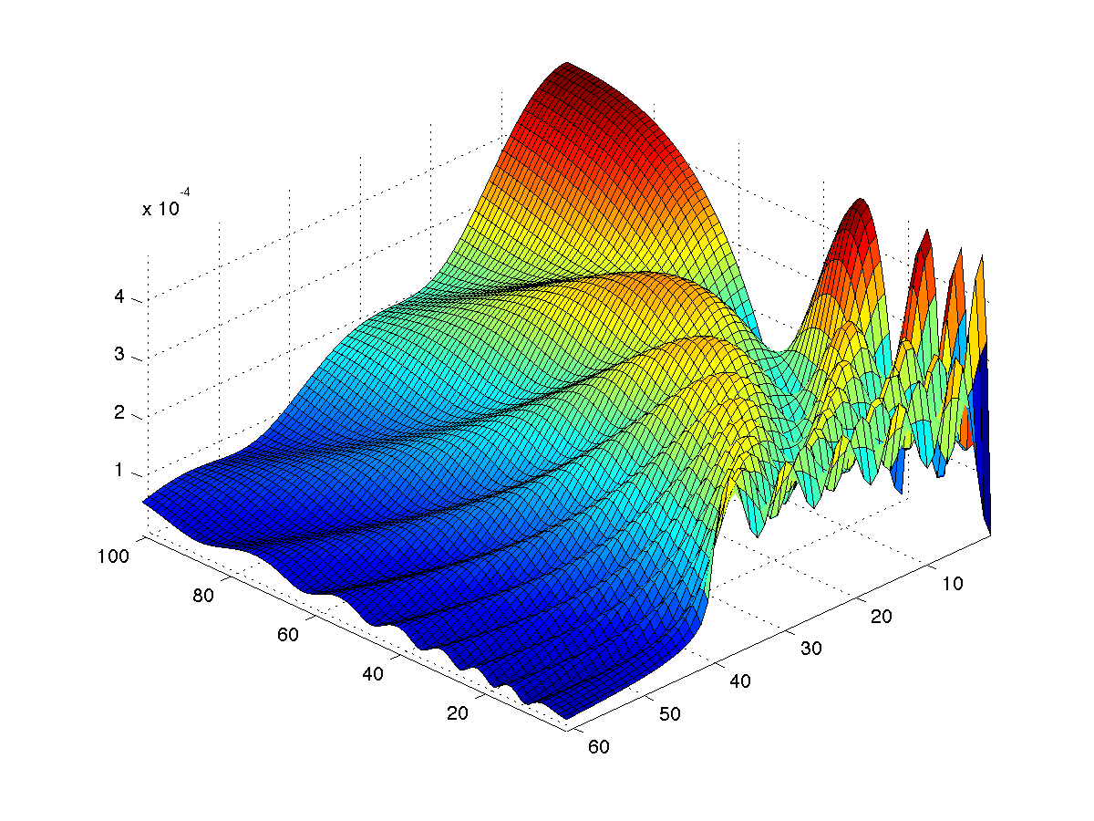
which should result in a picture file called "figure2.png" that looks as follows:define_media;
lambda = lossless.soundspeed/f0;
radius=5.0*lambda;
siz = [61 1 101];
sampling = [1.5*radius/(siz(1)-1) 1 radius^2/lambda/(siz(3)-1)];
ps=set_coordinate_grid(sampling,0,sampling(1)*(siz(1)-1),0,0,0,sampling(3)*(siz(3)-1));
transducer=get_circ(radius, [0 0 0], [0 0 0]);
pressure=cpu_fnm_call(transducer,ps,lossless,40,f0,0);
figure(2); surf(abs(squeeze(pressure))); axis tight; view(225,45);
saveas(figure(2), 'figure2.png')
Regular Piston Arrays
Arrays of pistons are calculated by first computing a larger single-piston solution and then computing a convolution with the piston pattern. We start by computing the piston from above at an extended 256-wide grid and do a convolution in x direction, where each piston has a center-center distance to its neighbor of 64 grid points, i.e., 64/61*radius.
%% setup parameters
f0=1000000; % excitation frequency
c=1500; % speed of sound
lambda = c/f0; % wavelength
k=2*pi/lambda; % wavenumber
radius=5.0*lambda; % piston radius
siz = [ 256 1 101 ];
sampling = [1.5*radius/(61-1) 1 radius*radius/lambda/(siz(3)-1)];
transform = [ sampling(1) 0 0 0; 0 sampling(2) 0 0; 0 0 sampling(3) 0; 0 0 0 1 ];
%% compute a single piston
pressure = MLCircularPistonGrid( transform, siz, radius, k, 'cpu', 40);
figure(2); surf(abs(squeeze(pressure))); axis tight; view(225,45);
saveas(figure(2), 'figure2.png')
%% compute the convolution of four elements, triggered synchronously
array_pressure = MLRectilinearArrayConvolution( pressure, [1; 1; 1; 1], 4, 1, 64, 1, 'cuda')
%% draw figure
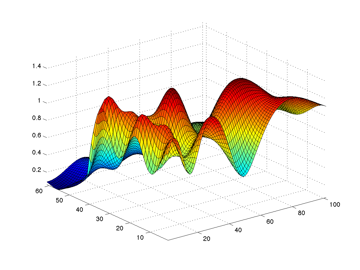
figure(3); surf(abs(squeeze(array_pressure))); axis tight; view(225,45);
saveas(figure(3), 'figure3.png');
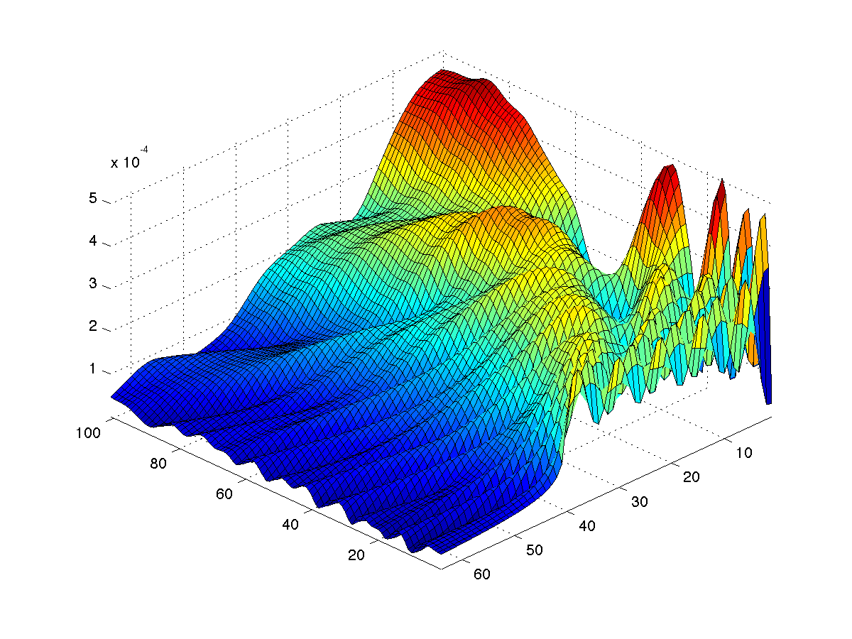
The result is a 64x1x101 grid that is aligned with the outer of the four pistons as shown here:f0=1000000; % excitation frequency
c=1500; % speed of sound
lambda = c/f0; % wavelength
k=2*pi/lambda; % wavenumber
radius=5.0*lambda; % piston radius
siz = [ 256 1 101 ];
sampling = [1.5*radius/(61-1) 1 radius*radius/lambda/(siz(3)-1)];
transform = [ sampling(1) 0 0 0; 0 sampling(2) 0 0; 0 0 sampling(3) 0; 0 0 0 1 ];
%% compute a single piston
pressure = MLCircularPistonGrid( transform, siz, radius, k, 'cpu', 40);
figure(2); surf(abs(squeeze(pressure))); axis tight; view(225,45);
saveas(figure(2), 'figure2.png')
%% compute the convolution of four elements, triggered synchronously
array_pressure = MLRectilinearArrayConvolution( pressure, [1; 1; 1; 1], 4, 1, 64, 1, 'cuda')
%% draw figure
figure(3); surf(abs(squeeze(array_pressure))); axis tight; view(225,45);
saveas(figure(3), 'figure3.png');
Keep in mind that any call to MATLAB involves copying data from MATLAB to C/C++ to the GPU. This may slow down some operations tremendously.